At a glanceAn #N/A error means Excel cannot find the specified value in the lookup range. This article outlines Microsoft’s recommended checks for XLOOKUP and VLOOKUP, using illustrative examples rather than a reproduced worksheet.
AI-generated editorial illustration; not a product screenshot.
An #N/A error in Excel means that the function cannot find the value it was instructed to look for in the lookup range. Based on Microsoft support documents, this article organizes the checks to make when XLOOKUP or VLOOKUP returns #N/A. The worksheet was not opened and tested directly, and the table and formulas below are hypothetical examples for illustration.
1. Check whether the lookup value actually exists in the source range
The most common cause is that the lookup value does not exist in the source data. For example, if the lookup value is “banana” but the price list has no banana row, VLOOKUP returns #N/A. Copy the value from the lookup cell and search for it in the source range with Ctrl+F. Even values that look identical may fail to match because of trailing spaces or different characters.
2. Match number and text formats and remove spaces
If the lookup value is a number but the value in the source table is stored as text, the two values may not be recognized as equal, resulting in #N/A. Microsoft’s documentation recommends checking the cell format first and, if necessary, shows an example of looking up a range with leading and trailing spaces removed using the TRIM function. Before changing the source column directly, it is safer to check the result in an adjacent column.
3. Confirm that the lookup is for an exact match
If the last argument of VLOOKUP is TRUE or omitted, it attempts to find an approximate match when no exactly matching value exists. This can produce #N/A, or an incorrect result even when the exact value exists. To find an exact match, use FALSE, as in =VLOOKUP(lookup_value, table_range, column_number, FALSE). XLOOKUP uses exact match by default, so this issue is less common, but it still returns #N/A when it cannot find a match.
4. Display a value only for rows that are legitimately missing
If an item is legitimately absent from the list, it is better to define the result in advance than to hide the error. In XLOOKUP, you can enter text such as “Not found” in the fourth argument, if_not_found. Example: =XLOOKUP(A2, code_column, name_column, "Not found"). XLOOKUP cannot be used in versions 2016 and 2019, so you can use IFNA to replace only #N/A, as in =IFNA(VLOOKUP(A2, table_range, 2, FALSE), "Not found"). Because IFERROR hides all errors, be careful not to conceal errors such as #REF! caused by an incorrect formula range.
5. Summary of the checking order
① Search for the lookup value in the source range. ② Check the number or text format and leading or trailing spaces. ③ Set the last argument of VLOOKUP to FALSE. ④ Add a label such as “Not found” only for rows that are legitimately missing. If the issue is still unresolved after these checks, finally verify that the range referenced by the formula is correct and that the sheet name has not changed.
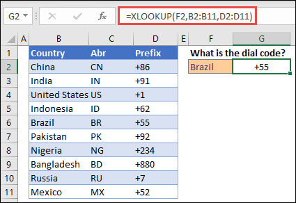
Microsoft Excel example: =XLOOKUP(F2,B2:B11,D2:D11) looks up Brazil in column B and returns +55 from column D. This demonstrates a successful match; check that your lookup value exists before handling #N/A. Source: Microsoft Support. Used with permission from Microsoft. Reuse terms.
This article reflects public information available when it was written. Specifications, prices and schedules can change; check the linked official documentation.
This English edition was written and translated with AI assistance, with sources provided. For errors or additional information, please request a correction. Editorial policy
Found this useful? Share it, or follow for new guides.
If an Excel total is 0 or numbers are aligned left, they may be stored as text. Based on Microsoft Support, this article explains how to check the display and convert them back to numbers.
When SUMIFS returns a #VALUE! error, first check that all ranges in the formula have the same number of rows and columns, as Microsoft Support explains for sum_range and criteria_range.
Learn how to create an Excel drop-down list with Data Validation, configure its source, and manage the list later based on Microsoft support documentation.